Squishy Images

I recently attended a southeastern photography society meeting which was neat. Many of the photographers lamented the demise of polaroid imaging. Apparently, there was quite a sub-culture involved in modifying the process either to put images on unusual papers or to modify SX-70 images while they were still squishy.

I loved the squishy effect and the applied mathematician in my background realized it was a problem in fluid dynamics. Therefore, it was something fun to play with and more importantly I knew how to do it.

Or at least I thought I did. Turning the idea into an algorithm and then an efficient program took a little work. Work which I’ll describe after the photots.

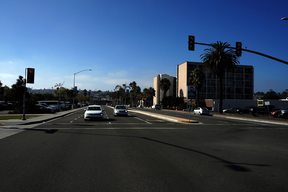
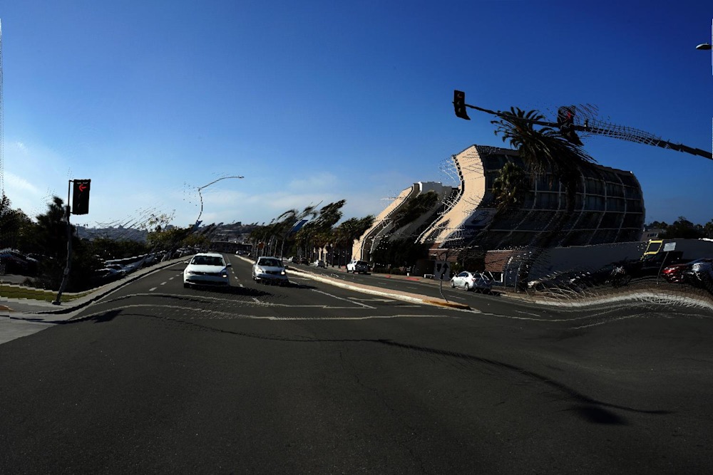
Here’s my test image. Nothing special, really, just a street scene in San Diego from a study section trip. 

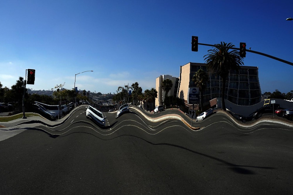
After applying a coordinate deformation, I generate this wavy image.  The coordinate deformation is determined by the red and green bits on an input mask:

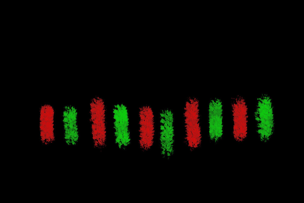
This is designed so you can use a layer in photoshop or Gimp to draw it over the original image. Red is high pressure, where the image moves away, and green is low pressure, where the image moves to.  The background can be black, white, or transparent without effect.

Using a different pattern results in a different image:

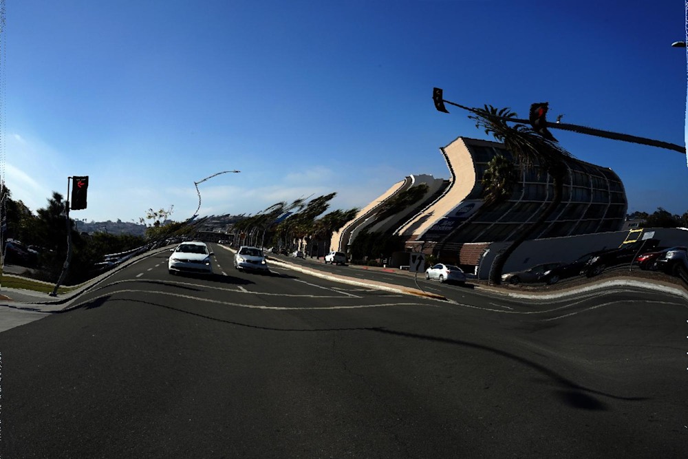
Which is sort of cool.

Outside of efficiency issues and wandering aimlessly down a quick and dirty approximation (never a good idea), the only real issue is mapping grids to grids when bending the surface coordinates. If the effects of mapping floating point numbers to integers is not corrected, the image degrades with lots of little bitsy things:

Eventually, those bitsy things take over the entire image, which is sort of ugly.

The algorithm involves inputting the initial pressure (that red/green map) and then solving for an equilibrium solution or potential. You can do this with finite differences but that is really really really slow. Instead I used a convolution with the scipy.signal.convolution function. It’s a bit tricky to figure out the reference frame for the convolution, but once understood and implemented correctly it’s blazingly fast.

I then find the gradient of that potential. Again, scipy.signal.convolution comes to the rescue as I define the finite element for the difference and simply convolve that with the potential. This is much easier done than said. (if you want to see the math, we developed it in detail for a related problem and on google scholar)  

The final issue is performing gradient descent in the image coordinate space. If you take an efficient sized step, then the integer round off when you map between the real value of the estimate and its closest integer will always skip a few pixels. Iterating this ends up with lots of additional little lines. So it is necessary to perform a smooth extension along the gradient by filling in with multiple step sizes (again easier to do than to say).